Comparing the incomparable — expanding the time map concept

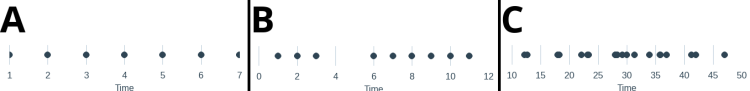
We are surrounded by discrete events: posts and comments, purchases from the online store, page visits are all examples of discrete events. Some of these events happen periodically; others happen sporadically. Some happen once in a while; others are generated every microsecond. There are many ways to visualise such streams, the most naive one being a one-dimensional plot in which events are placed on a time axis, as demonstrated in the figure below for three simple cases.

But what happens if there are too many such events? How do we gain a global overview? Recently, I have learned about “Time maps” — a creative way to perform such a visualization, which I will describe below using examples from WordPress.com. I will expand this approach to accommodate for bringing cases with drastically different time scales to the same domain, for easier comparison and pattern discovery.

Time maps

Instead of plotting the absolute time values, or time differences, Max Watson from District Data Labs suggests representing each data point in two dimensions — in terms of time passed before and after the events. Thus, all the data points from case A in the figure above will be represented by the pairs as all of them occur at regular intervals of 1 second. Most of the dots in case B from the same figure will be represented by the same pair, . However, the pause between the event at time marks 3 and 6 seconds and not 1. Thus, the third point will be represented by and the fourth one — by . Following are the time maps for the three toy cases from the figure above:

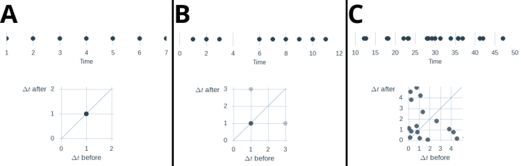
Note that all the dots in case A overlap. Now we can identify several interesting regions in these time maps. Events that happen at equal intervals lie on the diagonal line and overlap. Events that occur at approximately equal intervals will be distributed over the diagonal. The upper right portion of the map represent events that happen at a slow pace while the lower-left quadrant of the graph represents fast events. Long interruptions followed by recovery manifest as large deviations from the diagonal — the interruption itself (high ) is shown as a dot above the diagonal and the event after the interruption (high ) appears as a dot to the right of the diagonal.

Let us examine some real-life events. I’ll start with publishing posts or pages on some of the WordPress.com blogs.

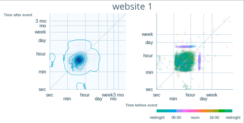
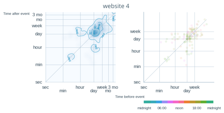
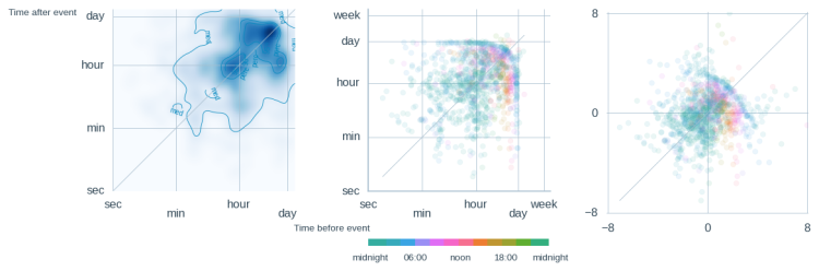
Following is a time map of a particularly busy site with more than 7,700 posts. On the right, you may see post and pages time map in which each point is colored according to the GMT in which the post was published. Note the logarithmic scale of the plot that shows events at time intervals of several orders of magnitude — from seconds to weeks. As you may see, the vast majority of publishing events occur at intervals of several minutes to one hour. The lines of purple dots represent breaks of approximately eight hours in publishing new posts — something that is consistent with a medium size editorial team. To the right, I present a landscape representation of the same time map. The dark blue bulb in the graph on the left shows that the vast majority of the events occur at regular intervals between several minutes and one hour.

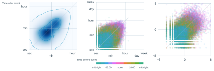
Time map of another busy site, with its 6511 posting events, shows a slightly different publishing pattern.

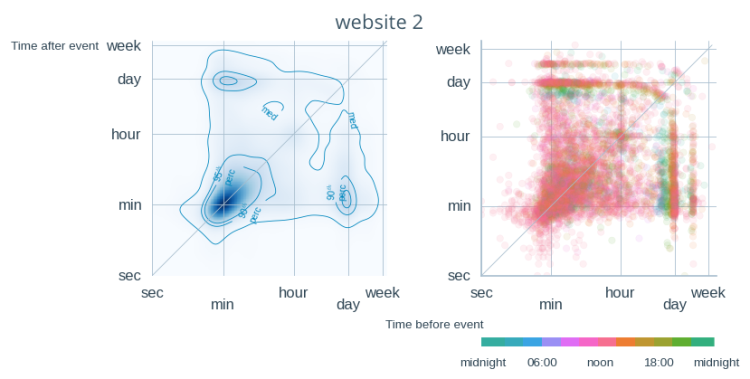
In this news site, most of the events occurred at one-minute intervals. The typical service break in this site is either one or two days long, as represented by the two distinct strips.
Using the time map approach is relatively easy to identify bots. For example, the owners of the following site have uploaded more than 1,000 posts such that most of them were published at a one-minute interval — a pattern that is unlikely to be performed by a human.

What about smaller blogs? This Norwegian blogger posted less than 150 posts with a typical time interval between a day and week.

I have analyzed time maps of different administrative tasks performed by  several random WordPress.com users.
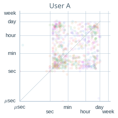
This user, for example, is a moderately active blogger with a single blog. Their time map is characteristic of sporadic events with intervals of several seconds to one day. We may see that this user is very disciplined and does not leave the blog for more than a day.

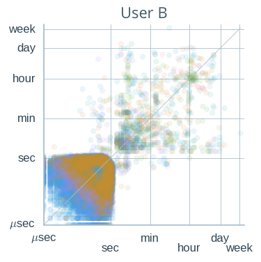
On the other hand, another user, who has two blogs presents a completely different time map with thousands of events within the range of micro- and milliseconds. Notice that the two types of events (the super-fast ones and the “normally paced” ones) are well separated and that the super-fast events occur at very specific hours. Does this mean that that user’s computer is affected by a virus? Does that user use an aggressive script to monitor their site? This is a topic for another post.

 

Bringing the maps to the common scale

You may have noticed the vast differences in time scales that we saw in the maps above. Sometimes, we are interested in map’s shape, so that we can compare similar patterns that occur at different time scales. To achieve this task, I first sort time difference values in each case (user, blog, log record, etc.). Next, I transform these values such that the median time difference (the one that is larger than half of the observed points) gets the value of 0. Time differences larger then the median receive positive values and time differences smaller than the median receive negative values. In technical terms: I first compute the empirical cumulative distribution of the time differences, and then perform logit transform.

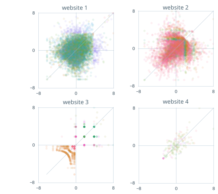
The following figure shows the normalised maps for four blogs I have mentioned at the beginning of this document . We may see that the elliptical shape of the dot cloud represents a series of events that occur somewhat regularly at a relatively low frequency. Round-shaped graphs represent cases in which the typical variability in inter-event periods is comparable to that period. Bot-induced time maps are still easily detected in this representation

Let us now examine the normalised time maps of the two users mentioned above:

One interesting thing to note is the fact that the lower-left region in the second user’s graph is now significantly enlarged because it contains a much larger amount of data points. As with the case of the blog time maps, the approximately round shape of the first user’s time map indicates that the variability of the between-event interval is comparable in its size to the interval. Note, though, that when observing first user’s raw map, it was clear that that user’s events mostly occur not faster than once a second, and that there the maximal interval is never larger than one day. Such a notion, which may be valuable in many cases, is absent from the normalised graph.

Conclusions

Time maps, as developed by Max Watson from District Data Labs provide a valuable insight in the analysis of event streams. It is evident that these maps reveal interesting activity patterns. Analysis of such patterns may be used in spam and fraud detection.

The proposed normalisation of time maps provides a tool for comparing the shapes of drastically different maps. The following figure, for example, presents time maps of Premium and Business purchases performed in Japanese Yens between June 1st and Dec 20th, 2015 :.

I selected the Yen as the least frequent currency used in WordPress.com. Had I analysed the same data for USD, we would see a completely different raw map, but comparable normalised one: